Barton Journal

FULL-LENGTH ARTICLE

Morgan Cassell*, Ashley L. Bennett⁺, and Nicole L. Mazuroski⁺

School of Health Sciences, Barton College, Wilson, NC, USA
*Student author, ⁺Faculty mentor

---

CITATION

Cassell, Morgan; Bennett, Ashley L.; & Mazuroski, Nicole L. (2026). A mathematical approach to prion misfolding. Barton Journal, 1(1), 47–71. https://bartonjournal.org/vol-1-no-1/2026-cat1-article-no-002

---

 Abstract 

Prion diseases are a rare form of infectious neurodegenerative disorders that can infect humans as well as other mammals and can also be transferred from mammals to humans. Currently, these  prion diseases remain both fatal and untreatable. These serious prion diseases are ultimately caused by the transformation of the prion protein (PrPᶜ), which is natively expressed in the central nervous system of mammals, into an infectious isoform, PrPˢᶜ. High resolution NMR and cryo EM structures of PrPᶜ and PrPˢᶜ have revealed vast structural differences between the two isoforms despite having the same amino acid sequence. While much is known about the specific structural differences between the native and infectious PrP isoforms, almost nothing is understood about the initial misfolding events triggering the PrPᶜ to fold into the PrPˢᶜ or the specific details of how a misfolded PrPˢᶜ infectious isoform and trigger a non-infectious PrPᶜ into the infectious isoform. Here, we provide a mathematical framework for studying prion structures and folding with the goal of building a predictive model. Leveraging experimentally derived constraints we demonstrate a topology-based model that enables a dimensionality reduction of the coordinate space by projection onto the contact space, thus enabling more efficient analysis of the interacting residues and interactions driving the PrPᶜ misfolding to PrPˢᶜ.  Now that this framework is established, we will integrate with biophysical,  structural, and machine learning analyses to explore the cellular factors that act as predictors for triggering a prion protein misfolding event. 

Keywords: prion diseases, protein misfolding, prion protein, neurodegenerative disorders,  mathematical modeling, topology, dimensionality reduction, contact space analysis, structural  biology

---

Introduction 

Prion diseases are a class of transmissible neurodegenerative disorders affecting a wide range of mammalian species. Human-specific prion diseases include Creutzfeldt-Jakob Disease  (CDJ), Kuru, or Fatal Familial Insomnia (FFI) and remain untreatable and fatal. Prion diseases result when a transmutation of PrPᶜ, which is natively expressed in neurological tissue in mammals, is transformed into the infectious isoform, PrPˢᶜ. Aggregation of the prion misfold causes a rapid deterioration of the neuron expressing fibril chains of PrPˢᶜ (Miranzadeh  Mahabadi & Taghibiglou, 2020).  

Much like a viral disease, PrPˢᶜ ultimately spreads and infects other nervous tissue in the central nervous system (CNS) of any host mammal. Although both isoforms share identical primary amino acid sequences consisting of approximately 210 residues after post-translational processing, where the difference lies in secondary and tertiary structure, resulting in a distinct fold between the two isoforms. PrPᶜ adopts a globular fold containing three 𝑎-helices and two short 𝛽-sheets while PrPˢᶜ adopts a 𝛽-sheet rich fibrillar architecture, typically forming parallel,  in-register 𝛽-sheets (Kovač & Čurin Šerbec, 2022; Kraus et al., 2021; Wille & Requena,  2018). Structural studies have identified structural variability in the 𝛽2–𝑎2 loop (residues 165- 175) and the 𝑎2–𝑎3 interhelical interface (residues 185-209), regions that are implicated in the transition from PrPᶜ to PrPˢᶜ (Kraus et al., 2021). These regions provide plausible candidates for residue pairs (i′, j′) that contribute to the distance discrepancies between corresponding residue pairs, which can be measured with contact graphs and their threshold proximities. Residue pairs that show the largest differences in the contact maps are potential candidates for driving the misfold and structural separation between PrPᶜ and PrPˢᶜ. 

Prion proteins can take on many variations with one example being 1FO7, which is a  mutant fragment from residues 90-231 containing 60 total conformations calculated, 30 of which  have been verified and submitted. The same is true for a mammalian vector such as the Syrian  Hamster (M. auratus), which examines residues 90-231 and has 100 calculated structures, 25 of which confirm the overall structural conformation of 2 𝛽-sheets and 3 𝑎-helices with sequences binding the 5 main structures of the globular domain.  

The precise mechanism of this structural transition remains incompletely understood. This paper integrates topological and distance-geometric analyses to reveal the mechanism(s) of  PrPᶜ and its infectious isoform PrPˢᶜ. Subsequent stereochemical and structural analysis is used to map mathematical findings to the protein structures and reveal the underlying residue interactions driving prion protein misfolding. 

Mathematical Methodology

The primary aim is to demonstrate through proof that a transformation from PrPᶜ to PrPˢᶜ is defined and then map the mathematical transformation onto the prion protein isoform  structures. While the real-world infectivity of the PrPˢᶜ protein misfold is known, much is left  unknown about misfolding initiating and propagation mechanisms. Resolving these mechanisms  of pathogenesis requires a fresh perspective. We provide a mathematical model of structural  transformation for representative prion protein structures 1QLX and 6LNI in ℝ¹, ℝ², and  ℝ³ representing sequence, contacts, and coordinate space, respectively. Given that we need a  concrete and strong initial base, we can break down the analysis into multiple categories of  application.

 Proof in ℝ¹ 

Axiom 1: 

Let ∑ denotate the 20-letter amino acid alphabet. Post-enzymatic trimming, a mature PrP consists of 210 amino acid sequences. Therefore the sequence space is defined as; 

𝑆 = ∑²¹⁰ where, ∑²¹⁰ = {𝑎ᵢ ∈ ∑ | (𝑎₁, 𝑎₂, 𝑎₃, … , 𝑎₂₁₀) }. 

In addition, there does exist some 𝑠 ∈ 𝑆 which represents an ordered 210-residue sequence.

Axiom 2: 

Let 𝐽: 𝑆 → 𝑌 be an invariant and define a relation ~ᴊ on 𝑆 by: 

𝑠 ~ᴊ 𝑡 ⟺ 𝐽(𝑠) = 𝐽(𝑡) 

Lemma 1: Invariant-Induced Relations is an Equivalence Relation. 

Claim: For any function 𝐽: 𝑆 → 𝑌, the relation ~ᴊ is an equivalence relation on 𝑆.

Proof: Define the following terms:

i. Reflexivity: ∃𝑎 such that, 𝑎 = 𝑎
ii. Symmetry: ∃𝑎, 𝑏 such that, 𝑎 = 𝑏 & 𝑏 = 𝑎
iii. Transitivity: ∃𝑎, 𝑏, 𝑐 such that, 𝑎 = 𝑏 and 𝑏 = 𝑐 ⟹ 𝑎 = 𝑐. 

Projecting these terms onto the initial claim results in:

i. If 𝐽(𝑠) = 𝐽(𝑠), then 𝑠 ~ᴊ 𝑠
ii. If 𝐽(𝑠) = 𝐽(𝑡), then 𝐽(𝑡) = 𝐽(𝑠)
iii. If 𝐽(𝑠) = 𝐽(𝑡) and 𝐽(𝑡) = 𝐽(𝑢), then 𝐽(𝑠) = 𝐽(𝑢) .

Which then implies ~ᴊ is reflexive, symmetric, and transitive. ∎

Axiom 3: 

Define the identity invariance as: 

𝐽₁: 𝑆 → 𝑆, 𝐽₁(𝑠) = 𝑠, 

Then the relation will satisfy: 

𝑠 ~ᴊ₁𝑡 ⟺ 𝑠 = 𝑡. 

Because the prion conversion from globular PrPᶜ to infectious isoform PrPˢᶜ is solely a conformational change and not a sequence or residue change, we can establish that the sequence is preserved regardless of conformational change. So, if we take some sequence: 

𝑠꜀, 𝑠ₛ꜀ ∈ 𝑆

Then the mature sequence residues will exist as: 

𝑠꜀ = 𝑠ₛ꜀. 

Theorem 1: PrP Sequence Indistinguishability 

Claim: under the primary invariance 𝐽₁, PrPᶜ and PrPˢᶜ lie on the same equivalence class  𝑆 ⁄ ~ᴊ₁. 

Since: 𝑠꜀ = 𝑠ₛ꜀ we can say: 

𝐽₁(𝑠꜀) = 𝑠꜀ = 𝑠ₛ꜀  = 𝐽₁(𝑠ₛ꜀ ) 

⟹ 𝐽₁(𝑠꜀) = 𝐽₁(𝑠ₛ꜀ ) 

⟹ 𝑠꜀ ~ᴊ₁ 𝑠ₛ꜀ 

⟹ [𝑠꜀]ᴊ₁ = [𝑠ₛ꜀ ]ᴊ₁ ∎

Corollary for Theorem 1: Failure of Sequence-Level Detection Must Exist 

Claim: no invariant depending solely on primary sequence identity can distinguish PrPᶜ from PrPˢᶜ. 

Since: 𝑠꜀ = 𝑠ₛ꜀ we can use direct substitution to impose: 

⟹ 𝐽(𝑠꜀) = 𝐽(𝑠ₛ꜀). 

Therefore, if every invariant is defined solely on a primary sequence PrP which is contained in the enzymatic trimmed chain ∑²¹⁰, then both PrPᶜ and PrPˢᶜ are indistinguishable. This is further elaborated in the biological perspective in which the PrP parent chain can be expressed either as the infectious fibril misfold or the native globular protein. Thus: 

(PrPᶜ = PrPˢᶜ) ⊂ ℝ¹ ∎

Because experimentally we know that a misfold occurs somewhere in the protein life cycle, we are going to assume that fact and proceed forward in a fashion that emphasizes  mathematical perspective. The goal is to then prove the non-congruence of PrPᶜ and PrPˢᶜ in ℝ² and ℝ³. As shown above, the ℝ¹ sequence space is congruent in residue sequence, however the two isoforms are known to be non-congruent in conformation. As the conformational ℝ³ space is better described experimentally than the ℝ² contact space, the proof in ℝ³ will be written first to easily observe the difference in structural conformation. That difference or conformational change in structure will be more easily presented through contact maps in the ℝ² proof.

 Proof in ℝ³

Axiom 4: Index Set 

Let 𝐼 be a finite residue index set on which both coordinate models supply. Concretely, 𝐼 is taken to be the intersection of the residue indices present in: 

• PrPᶜ, which exists as a globular C-terminal domain and has 3 𝑎-Helices and a short β sheet 
• PrPˢᶜ, presents parallel in-register intermolecular β-sheets 

𝐼 = (𝐶) ∩ (𝑆𝑐). 

Defining 𝐼 as the overlap avoids any non-trivial index matching assumptions beyond the correlation to coordinates and labeled residues. 

Axiom 5: Projection Mapping 

Fix a representative atom per residue then define the embeddings as: 

𝐹𝑐:𝐼 → ℝ³, 𝐹𝑠𝑐:𝐼 → ℝ³ 

Where 𝐹𝑐(𝑖) and 𝐹𝑠𝑐(𝑖) be the 3D coordinates of the mmCIF atoms for the common residues in  1QLX and 6LNI, representing PrPᶜ and PrPˢᶜ, respectively. 

Axiom 6: Rigid Motion 

A rigid motion in ℝ³ specifically is a representative mapping in form: 

𝑔(𝑥) = 𝑅𝑥 + 𝑣, 𝑅 ∈ 𝑂(3), 𝑣 ∈ ℝ³.

Where the matrix 𝑅 belongs to the orthogonal group 𝑂(3), defined as: 

𝑂(3) = {ℝ ∈ ℝ³ˣ³| 𝑅ᵀ𝑅 = 𝐼} 

The main advantage of orthogonal matrices is that they preserve Euclidean inner product and thus lengths and pairwise distances. Consequently, any transformation of the form 𝑔(𝑥) = 𝑅𝑥 + 𝑣 where 𝑅 ∈ 𝑂(3) and 𝑣 ∈ ℝ³ is a Euclidean isometry of ℝ³. Distance matrices are therefore invariant under such transformations. 

Axiom 7: Euclidean Congruence 

Define 𝐹𝑐 and 𝐹𝑠𝑐 as congruent if there exists a rigid motion 𝑔 such that: 

𝐹𝑠𝑐(𝑖) = 𝑔(𝐹𝑐(𝑖)), ∀𝑖 ∈ 𝐼

Axiom 8: Distance Matrix on an Embedding 

For an embedding in the projection 𝐹:𝐼 → ℝ3, define its distance matrix 𝐷ꜰ such that:

𝐷ꜰ:𝐼 × 𝐼 → ℝ≥₀, 𝐷ꜰ(𝑖,𝑗) = ‖𝐹(𝑖) − 𝐹(𝑗)‖. 

Given the following axioms, we can begin to establish lemmas 2 and 3 which state claims  that rigid motion preserves pairwise distance, which was previously assumed in axiom 7 as well  as a contrapositive separation. 

Lemma 2: Rigid Motion Preserves Pairwise Distance 

Claim: if 𝐹𝑠𝑐 = 𝑔(𝐹𝑐) for a rigid motion 𝑔 then: 

𝐷ꜰₛ꜀ (𝑖,𝑗) = 𝐷ꜰ꜀ (𝑖,𝑗), ∀𝑖,𝑗 ∈ 𝐼. 

Proof: ∀𝑖,𝑗 ∈ 𝐼: 

𝐷ꜰₛ꜀ (𝑖,𝑗) = ‖𝐹𝑠𝑐(𝑖) − 𝐹𝑠𝑐(𝑗)‖ = ‖𝑔(𝐹𝑠𝑐(𝑖)) − 𝑔(𝐹𝑠𝑐(𝑗))‖. 

Given axiom 7 we can establish 𝑔(𝑥) = 𝑅𝑥 + 𝑣 with 𝑅 ∈ 𝑂(3) such that:

‖𝑔(𝑎) − 𝑔(𝑏)‖ = ‖𝑅(𝑎 − 𝑏)‖ = ‖𝑎 − 𝑏‖. 

Therefore:  

𝐷ꜰₛ꜀ (𝑖,𝑗) = ‖𝐹𝑠𝑐(𝑖) − 𝐹𝑠𝑐(𝑗)‖ = ‖(𝑅𝐹𝑐(𝑖) + 𝑣) − (𝑅𝐹𝑐(𝑗) + 𝑣)‖ = ‖𝑅(𝐹𝑐(𝑖) − 𝐹𝑐(𝑗))‖ = ‖𝐹𝑐(𝑖) − 𝐹𝑐(𝑗)‖ = 𝐷ꜰₛ꜀ (𝑖,𝑗) ∎

Lemma 3: Contrapositive Separation 

Claim: If there exists a pair 𝑖,𝑗 ∈ 𝐼 such that: 

𝐷ꜰₛ꜀ (𝑖,𝑗) ≠ 𝐷ꜰ꜀(𝑖,𝑗), 

then there is no rigid motion 𝑔 where 𝐹𝑠𝑐 = 𝑔(𝐹𝑐). 

Proof: If lemma 2 holds true that if rigid motion 𝑔 exists with 𝐹𝑠𝑐 = 𝑔(𝐹𝑐), then all  corresponding pairwise distances must agree:  

𝐷ꜰₛ꜀ (𝑖,𝑗) = 𝐷ꜰ꜀(𝑖,𝑗), ∀𝑖,𝑗 ∈ 𝐼. 

Which is the implicit contrapositive of lemma 2 and thus if even 1 pair of residues satisfies:

𝐷ꜰₛ꜀ (𝑖,𝑗) ≠ 𝐷ꜰ꜀(𝑖,𝑗) 

Then the embeddings cannot be related by any rigid motion. Therefore, 𝐹𝑠𝑐 and 𝐹𝑐 are not Euclidean-congruent. ∎

This, however, is not sufficient evidence alone to establish a loose non-congruence of  Euclidean space structures; there must be a witnessed pair that either one structure has, but the other one does not. 

Axiom 9: Supremum of Distance Matrixes 

Define the discrepancy between the two embeddings by the following: 

Δ∞(𝐹𝑐, 𝐹𝑠𝑐) = |𝐷ꜰ꜀ (𝑖,𝑗) − 𝐷ꜰₛ꜀ (𝑖,𝑗)|. 

Since 𝐼 is a finite set, this maximum will exist. This quantity represents the largest pairwise distance disagreement between the two respective embeddings. 

Theorem 2: ℝ³ Non-Congruence Explicit 

Claim: From experimental data we assume: 

Δ∞(𝐹𝑐, 𝐹𝑠𝑐) > 0

Therefore, there exists no rigid motion: 

𝑔(𝑥) = 𝑅𝑥 + 𝑣, 𝑅 ∈ 𝑂(3),  

such that: 

𝐹𝑠𝑐 = 𝑔(𝐹𝑐). 

Proof: If the embeddings were Euclidean congruent, then by Lemma 2: 

𝐷ꜰₛ꜀ (𝑖,𝑗) = 𝐷ꜰ꜀ (𝑖,𝑗), ∀𝑖,𝑗 ∈ 𝐼

⟹ Δ∞(𝐹𝑐, 𝐹𝑠𝑐) = 0.

This contradicts the experimentally derived assumption that Δ∞(𝐹𝑐, 𝐹𝑠𝑐) > 0 and thus implies that there exist no rigid motion mapping 𝐹𝑐 to 𝐹𝑠𝑐. ∎

We then need to construct a witnessed pair that exists as the set’s maximum pair, so we  then define: 

(𝑖’,𝑗’) ∈ 𝐼 × 𝐼

Such that: 

Δ∞(𝐹𝑐, 𝐹𝑠𝑐) = |𝐷ꜰ꜀(𝑖’,𝑗’) − 𝐷ꜰₛ꜀ (𝑖’,𝑗’)| 

This identifies residues whose specific spatial separation has the largest discrepancy between the  two embeddings. Thus: 

𝐷ꜰ꜀ (𝑖’,𝑗’) ≠ 𝐷ꜰₛ꜀ (𝑖’,𝑗’), 

which confirms an explicit geometric witness of the non-congruence between PrPᶜ and PrPˢᶜ. To further strengthen the above theories and lemmas we will construct a contact graph. 

Axiom 10: Contact Graph by an Embedding 

Let the function 𝐹 be defined as the projection of 𝐼 onto real space: 

𝐹:𝐼 → ℝ³ 

Where 𝐼 is an embedding of a finite index set, as previously stated. This allows for any fixed  threshold δ > 0 to define the graph 𝐺(𝐹, δ) with edge set 𝐸(𝐹, δ) such that: 

𝐺(𝐹, δ) = (𝐼, 𝐸(𝐹, δ)),

Where:

 (𝑖,𝑗) ∈ 𝐸(𝐹, δ) ⟺ ‖𝐹(𝑖) − 𝐹(𝑗)‖ ≤ δ and |𝑖 − 𝑗| > 2. 

Theorem 3: Separation of Contact Graphs 

Claim: If: 

Δ∞(𝐹𝑐, 𝐹𝑠𝑐) > 0, 

then ∃δ > 0, such that: 

𝐺(𝐹𝑐, δ) ≠ 𝐺(𝐹𝑠𝑐, δ). 

Proof: Because we know from the experimental assumption:

Δ∞(𝐹𝑐, 𝐹𝑠𝑐) > 0, 

then there exist a witnessed pair such that: 

𝐷ꜰ꜀ (𝑖’,𝑗’) ≠ 𝐷ꜰₛ꜀ (𝑖’,𝑗’). 

So, without loss of generality, we can assume: 

𝐷ꜰ꜀ (𝑖’,𝑗’) < 𝐷ꜰₛ꜀  (𝑖’,𝑗’). 

We will choose a δ such that: 

δ = . 

This then implies the following transformations: 

𝐷ꜰ꜀ (𝑖’,𝑗’) ≤ δ < 𝐷ꜰₛ꜀ (𝑖’,𝑗’) 

⟹ (𝑖’,𝑗’) ∈ 𝐸(𝐹𝑐, δ) and ∄(𝑖’,𝑗’) ∈ 𝐸(𝐹𝑠𝑐, δ) 

∴ 𝐸(𝐹𝑐, δ) ≠ 𝐸(𝐹𝑠𝑐, δ)

⟹ 𝐺(𝐹𝑐, δ) ≠ 𝐺(𝐹𝑠𝑐, δ). ∎

This establishes that there exists at least one witnessed pair (𝑖’,𝑗’) that belongs to one edge set but not the other, which implies that the corresponding contact graphs are non-congruent. To further this idea if we take into account the findings of Miranzadeh Mahabadi &  Taghibiglou (2020), then we can observe that conformational misfolds of PrPᶜ → PrPˢᶜ lies within the β2-𝑎2 loop region (residues 165–175), and the 𝑎2-𝑎3 inter-helical interfaces (residues  185–200) of PrPᶜ. 

Proof in ℝ² 

Axiom 11: Orthogonal Planar Projections 

Retain the same embeddings from the proof in ℝ³ and with the same embeddings  allowing 𝐼 to be a finite index set of the specific PrP parent chain sequence: 

𝐹𝑐, 𝐹𝑠𝑐: 𝐼 → ℝ³. 

If we then define 3 standard orthogonal planar projections, such that for any orthogonal  projection denoted 𝑂 can be represented as: 

𝑂𝑥𝑦(𝑥, 𝑦, 𝑧) = (𝑥, 𝑦), 𝑂𝑥𝑧(𝑥, 𝑦, 𝑧) = (𝑥, 𝑧), 𝑂𝑦𝑧(𝑥, 𝑦, 𝑧) = (𝑦, 𝑧). 

This reduction of geometric space gives 3 possible geometric planes as a result of each 𝑂𝑎,𝑏: ℝ³ → ℝ², which is a linear mapping of ℝ³ → ℝ² created by deleting a single coordinate.  

Axiom 12: Distance Structure Under Planar Projection

We can further define this mapping such that for any planar projection 𝐹:𝐼 → ℝ² we  define the embedding as: 

𝐷ꜰ(𝑖,𝑗) = ‖𝐹(𝑖) − 𝐹(𝑗)‖, 

where the double brackets denote the Euclidean norm on ℝ², which is: 

‖𝑥‖ = , ∈ ℝ². 

Additionally, we state that for 𝑃 ∈ {𝑂𝑥𝑦,𝑂𝑥𝑧, 𝑂𝑦𝑧}: 

𝐷 (𝑖,𝑗) = ‖𝑃(𝐹𝑐(𝑖) − 𝐹𝑐(𝐹𝑐))‖, 𝐷 (𝑖,𝑗) = ‖𝑃(𝐹𝑠𝑐(𝑖) − 𝐹𝑠𝑐(𝑗))‖.

Axiom 13: Threshold Contact Graph on Planar Projections 

To define the threshold graph on this 2-dimensional plane, we need to show that there exists some δ > 0 such that: 

𝐺(𝐹, δ) = (𝐼, 𝐸(𝐹, δ)), 

where some ordered pair (𝑖,𝑗) ∈ 𝐼 can be defined as: 

(𝑖,𝑗) ⊂ 𝐸(𝐹, δ) ⟺ ‖𝐹(𝑖) − 𝐹(𝑗)‖ ≤ δ and |𝑖 − 𝑗| > 2. 

Lemma 4: Projection Identities 

Claim: let there exist some vector ω such that ω = (𝑥, 𝑦, 𝑧) ∈ ℝ³, then we can show:

‖𝑂𝑥𝑦(ω)‖²+ ‖𝑂𝑥𝑧(ω)‖² + ‖𝑂𝑦𝑧(ω)‖² = 2‖ω‖². 

Proof: ω = (𝑥, 𝑦, 𝑧), which implies the following cases: 

𝑂𝑥𝑦(ω) = (𝑥, 𝑦), 𝑂𝑥𝑧(ω) = (𝑥, 𝑧), 𝑂𝑦𝑧(ω) = (𝑦, 𝑧)

⟹ ‖𝑂𝑥𝑦(ω)‖²= 𝑥² + 𝑦² 

⟹ ‖𝑂𝑥𝑧(ω)‖² = 𝑥² + 𝑧² 

⟹ ‖𝑂𝑦𝑧(ω)‖²= 𝑦² + 𝑧². 

This then give us: 

(𝑥² + 𝑦²) + (𝑥² + 𝑧²) + (𝑦² + 𝑧²) 

⟹ 2𝑥² + 2𝑦² + 2𝑧² 

⟹ 2(𝑥² + 𝑦² + 𝑧²) 

The internal portion of this product can be identified as the Euclidean norm in ℝ³, which  brings us back to our original vector that was proposed so we can conclude that: 

𝑥² + 𝑦² + 𝑧² = ‖ω‖² ⟹ 2(𝑥² + 𝑦² + 𝑧²) = 2‖ω‖² 

∴ ‖𝑂𝑥𝑦(ω)‖²+ ‖𝑂𝑥𝑧(ω)‖² + ‖𝑂𝑦𝑧(ω)‖²= 2‖ω‖² ∎

Lemma 5: Imposed Witness to Projection Identities 

Claim: using the same pair of witnessed points (𝑖’,𝑗’) ∈ 𝐼 such that the witnessed points  must exist in one plane or the other, allowing us to say: 

‖𝐹𝑐(𝑖′) − 𝐹𝑐(𝑗′)‖ ≠ ‖𝐹𝑠𝑐(𝑖′) − 𝐹𝑠𝑐(𝑗′)‖ 

⟹ ∃𝑃 ∈ {𝑂𝑥𝑦,𝑂𝑥𝑧, 𝑂𝑦𝑧} such that, 

𝐷 (𝑖’,𝑗’) ≠ 𝐷 (𝑖’,𝑗’). 

Proof: denote vectors 𝑣 and 𝑢 such that:

𝑣 = 𝐹𝑐(𝑖′) − 𝐹𝑐(𝑗′), and 𝑢 = 𝐹𝑠𝑐(𝑖′) − 𝐹𝑠𝑐(𝑗′). 

Given the hypothesis, neither 𝑣 nor 𝑢 can equal each other so we state that both 𝑣 and 𝑢 are  unique vectors to the specific witnessed pair (𝑖’,𝑗’) thus: 

‖𝑣‖ ≠ ‖𝑢‖. 

To demonstrate this, we will assume a contradiction that all 3 projections give equal  distances on the plane: 

‖𝑂𝑥𝑦(𝑣)‖ = ‖𝑂𝑥𝑦(𝑢)‖, ‖𝑂𝑥𝑧(𝑣)‖ = ‖𝑂𝑥𝑧(𝑢)‖, ‖𝑂𝑦𝑧(𝑣)‖ = ‖𝑂𝑦𝑧(𝑢)‖.

Given lemma 4 we can then say: 

‖𝑂𝑥𝑦(𝑣)‖²+ ‖𝑂𝑥𝑧(𝑣)‖² + ‖𝑂𝑦𝑧(𝑣)‖²= ‖𝑂𝑥𝑦(𝑢)‖²+ ‖𝑂𝑥𝑧(𝑢)‖² + ‖𝑂𝑦𝑧(𝑢)‖²

⟹ 2‖𝑣‖² = 2‖𝑢‖² 

⟹ ‖𝑣‖ = ‖𝑢‖ 

Thus, we reach a contradiction, and this shows that at least one of the coordinate planar  projections must satisfy that: 

‖𝑃(𝑣)‖ ≠ ‖𝑃(𝑢)‖ 

⟹ 𝐷 (𝑖’,𝑗’) ≠ 𝐷 (𝑖’,𝑗’) 

for some unique projection 𝑃 ∈ {𝑂𝑥𝑦,𝑂𝑥𝑧, 𝑂𝑦𝑧}.∎

Theorem 4: Separating Planar Groups 

If there exist a witnessed pair (𝑖’,𝑗’) ∈ 𝐼 such that:

‖𝐹𝑐(𝑖’) − 𝐹𝑐(𝑗′)‖ ≠ ‖𝐹𝑠𝑐(𝑖’) − 𝐹𝑠𝑐(𝑗′)‖, 𝑃 ∈ {𝑂𝑥𝑦,𝑂𝑥𝑧, 𝑂𝑦𝑧} 

with a unique threshold δ > 0 such that: 

𝐺(, δ) ≠ 𝐺(, δ). 

Proof: Induce lemma 5 and then choose one of the 3 unique planar projections 𝑃:

𝐷 (𝑖’,𝑗’) ≠ 𝐷 (𝑖’,𝑗’). 

Without a loss of generality, we can assume: 

𝐷 (𝑖’,𝑗’) < 𝐷 (𝑖’,𝑗’).

We then take a δ by the midpoint threshold such that: 

δ =, 

which gives the statement: 

𝐷 (𝑖’,𝑗’) ≤ δ < 𝐷 (𝑖’,𝑗’) 

⟹ (𝑖’,𝑗’) ∈ 𝐸(, δ) 

⟹ (𝑖’,𝑗’) ∉ 𝐸(, δ). 

This then allows us to establish that the edge sets are not equal: 

𝐸(, δ) ≠ 𝐸(, δ) 

⟹ 𝐺(, δ) ≠ 𝐺(, δ)∎

With an established witnessed pair existing, we can say that on the ℝ2 plane, there is at  least one pair of coordinate projections that preserves distance inequality, as well as the threshold for that planar distance inequality produces graph separation. 

Application 

To demonstrate a provable and direct contact graph inequality, we need to interpret the proof through the biological context from which it was derived. The solution NMR structure  1QLX contains the experimentally determined 3D coordinates for globular PrPᶜ (Bank, 1999)  and, alternatively, the coordinates for misfolding amyloid fibril PrPˢᶜ are deposited in the high-resolution (2.70 Å ) cryogenic electron microscopy (cryo-EM) structure (Data, 2019). This amyloid structure is a parallel in-register intermolecular beta sheet stack or PIRIBS (Data, 2019;  Zahn et al., 2000). Several hypotheses propose mechanisms for both the initiating structural change within a neuron and the propagation of the infectious isoform. Here, we apply our mathematical framework with hopes to provide evidence in support of one of the plausible mechanisms of misfolding and infectivity. To do so we apply the previously derived theorems that explain ℝ² & ℝ³. 

Applied proof in ℝ¹ 

While the PrPᶜ and PrPˢᶜ proteins have the same amino acid sequence, there are some differences in the experimentally determined coordinate structure because of the protein purification process. Specifically, the prion protein purification protocol used to determine the  1QLX structure has a 17 amino acid residue N-terminal tail and a thrombin cleavage site engineered in. This engineered N-terminal sequence in PrPᶜ structure results in a direct  difference in the encoding between PrPᶜ and PrPˢᶜ such that there exist 2 N-terminal residues in the beginning of the 1QLX sequence as well as an N-terminus residue and C-terminal residue on  the 6LNI. To accommodate this artifactual sequence change, we limit our analysis to the shared set of residues. This reduces the core residue count from each chain of 210 on each respective protein down to 208. This then allows us to analyze the following sequence code for Major Prion  Protein (MPP): 

KKRPKPGGWNTGGSRYPGQGSPGGNRYPPQGGGGWGQPHGGGWGQPHGGGWGQPHGGGWGQPHGGGWGQGGGTHSQWNKPSKPKTNMKHMAGAAAAGAVVGGLGGYMLGSAMSRPIIHFGSDYEDRYYRENMHRYPNQVYYRPMDEYSNQNNFVHDCVNITIKQHTVTTTTKGENFTETDVKMMERVVEQMCITQYERESQAYYQRGS

To simplify the MPP residue chain into a more chewable or easily represented object, we  will simply use the sigma notation from the previous Proof in ℝ¹, 

𝑀𝑃𝑃 = ∑²⁰⁸, 

where we can then denote 6LNI and 1QLX proteins as a projected reduction of the MPP residues. Specifically, the initial G and S on 1QLX and the beginning M and ending S on 6LNI, which are the respective termini, are truncated, such that we can denote 1QLX as C for a  representation of PrPᶜ and 6LNI as Sc for PrPˢᶜ: 

𝐶: ∑²¹⁰ → ∑²⁰⁸, 𝐶 = {𝑎₃, 𝑎₄, 𝑎₅,… , 𝑎₂₀₈, 𝑎₂₀₉, 𝑎₂₁₀} 

𝑆𝑐: ∑²¹⁰ → ∑²⁰⁸, 𝑆𝑐 = {𝑎₂, 𝑎₃, 𝑎₄, … , 𝑎₂₀₇, 𝑎₂₀₈, 𝑎₂₀₉} 

This sequence only representation of MPP, which allows us to take the initial claim of 𝐶 = 𝑆𝑐. Since both sequence representations are now equal to MPP, we can use MP to represent MPP  such that the following is true:

𝑀𝑃 = 𝐶 = 𝑆𝑐 ∈ ∑²⁰⁸ 

We can then impose the identity invariant such that: 

𝐽₁: ∑²⁰⁸  → ∑²⁰⁸,  𝐽₁(𝑠) = 𝑠

⟹ 𝐽₁(𝐶) = 𝐶 = 𝑆𝑐 = 𝐽₁(𝑆𝑐) 

⟹ 𝐶 ~ᴊ₁ 𝑆𝑐 

⟹ [𝐶]ᴊ₁ = [𝑆𝑐]ᴊ₁, 

if and only if : 

𝑀𝑃 = 𝐶 = 𝑆𝑐 ∈ ∑²⁰⁸. 

It should be noted that, based on the raw sequence with no exception to internal residue and  considering the termini: 

𝐶 ≠ 𝑆𝑐 ∈ ∑²⁰⁸. ∎. 

Applied proof in ℝ³ 

To demonstrate Euclidean graph invariance, we select the witnessed pair of residues 176 and 190 between the 3D space of 6LNI and 1QLX because these pairs of residues confer not only a local witness of |𝑖 − 𝑗 | > 2 but also a non-local witness using some delta as an anchor point. 

Axiom 4: Re-applied

Let the index set be defined as the intersection of the structure coordinates of the residue  pair, such that: 

𝐼 = (𝐶) ∩ (𝑆𝑐). 

Limitations in current experimental structural biology lead to missing residue density in experimental PrP structures. Therefore, PDB structure representing 𝐶 and 𝑆𝑐 are incomplete. The  1QLX structure representing the PrPᶜ structure is missing residues 21-124 and 229-230 and thus contains coordinates for only the fragment 125-228, which is roughly the 104-count residue of the globular domain. The same exists for 6LNI where the fibril core exists as residues 170-229.  This gives the intersecting set of: 

𝐼 = (𝐶) ∩ (𝑆𝑐)

𝐶 = {125,… , 228}, 𝑆𝑐 = {170,… , 229} 

⟹ 𝐼 = (𝐶) ∩ (𝑆𝑐) = {170,… , 228} 

⟹ 𝐼 = |59|∎ 

We then apply the distance graph of any witnessed pair: 

𝑖,𝑗 ∈ 𝐼, |𝑖 − 𝑗| > 2, 

in which the witnessed pair of residues 𝑖,𝑗 exist within this 59-residue set. To show that the witnessed pair on both graphs is not equal, we use the residues 176 and 190 as the non-local witness such that (𝑖’,𝑗’) = (176, 190). This allows us to determine: 

|176 − 190| = 14 > 2.

To show that the pair is a non-local witness, we must project the coordinates of the witnessed pair to the distance graph. As is standard for structural biology analysis, we select the alpha carbon (𝑎-carbon) atoms after a structural alignment between 1QLX and 6LNI to represent each residue. For the PrPᶜ structure 1QLX: 

• Residue 176 ∈ (−10.486,−14.457,−1.843) 
• Residue 190 ∈ (−0.774, 1.083,−0.983). 

And for PrPˢᶜ structure 6LNI: 

• Residue 176 ∈ (205.776, 211.731, 243.361) 
• Residue 190 ∈ (179.099, 234.532, 241.349). 

To get the residue pair distance for the distance graph we use: 

𝐷ƒ(𝑖,𝑗) = 

⟹ 𝐷ꜰ꜀ (176, 190) = 

⟹ 𝐷ꜰ꜀ (176, 190) = ≈ 18.34541 Å. 

The standardized data structure for mmCIF atom coordinate files on the PDB enables us  to use a Python implementation to automate extraction of distances between the atoms and  therefore a more accurate Ångstrom (where Å equals 10⁻¹⁰m or one 10 billionth of a meter and a  carbon-to-carbon single bond is ~1.54Å) distance such that for 1QLX the distance projection is: 

𝐷ꜰ꜀ (176, 190) = 18.347626004 Å

To show that a graph invariance exists, we perform the same analysis for the PrPSc structure 6LNI: 

𝐷ꜰₛ꜀ 176, 190) =

⟹ 𝐷ꜰₛ꜀ (176, 190) = ≈ 35.15104. 

And with the same code implementation, we can observe the encoded distance exists as:

𝐷ꜰₛ꜀ (176, 190) = 35.151046556 Å 

This result demonstrates that not only does the distance graph of the witnessed non-local  pair not equal each other but also that the computed residue distances in PrPᶜ and PrPˢᶜ do not  equal each other. We can now say that: 

𝐷ꜰₛ꜀ (176, 190) ≠ 𝐷ꜰ꜀ (176,190) 

This shows that no rigid motion exists in the contact graph. To further prove the two embeddings  are not equal we can take the midpoint δ > 0, which was defined in the proof, and compute the  midpoint threshold such that: 

δ = = 26.749336280 Å.

And if, 

𝐷ꜰ꜀ (176, 190) ≤ δ < 𝐷ꜰₛ꜀ (176, 190), 

then we can determine: 

(176, 190) ∈ 𝐸(𝐹𝑐, δ) and (176, 190) ∉ 𝐸(𝐹𝑠𝑐,δ) 

∴ 𝐺(𝐹𝑐, δ) ≠ 𝐺(𝐹𝑠𝑐, δ)∎

Using our implementation, we can automate this analysis over all combinations of residue pairs in the 59-residue intersection of the PrPᶜ and PrPˢᶜ structures, building a network graph for all possible witnessed local and non-local residue pairs (Figure 1). This comprehensive network graph demonstrates clearly that the edge set and the connectivity between the edges differ between the PrPᶜ and PrPˢᶜ structures. In the context of structural biology, this means that there are differences in the residues making up the edge sets and how the residues interact with each other in the two isoforms. 

Figure 1

Network Graphs of PrPᶜ and PrPˢᶜ

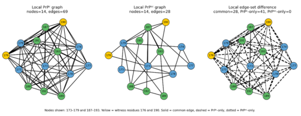
Note. Local network graphs for the intersecting  residue set 173–179 and 187–193 in (left) PrPᶜ, (middle) PrPˢᶜ, and (right) the difference between  PrPᶜ and PrPˢᶜ. The nodes represent the 𝑎-carbon atoms of the residues and the edges the  interactions between residues in the PrP structures. Yellow (176,190) represents the witnessed  pair selected during the application of the proof. In the panel on the right showing the edge set  differences, the solid lines show interactions in common between PrPᶜ and PrPˢᶜ, while the  dashed and dotted lines represent interactions that are present only in PrPᶜ or PrPˢᶜ, respectively.  

Applied proof in ℝ²

To show that there exists a unique orthogonal projection, we impose the same 𝑎-carbon  coordinates such that the difference between the unique witnessed pair (176, 190) would be: 

𝐹(176) − 𝐹(190) = (𝑥₁₇₆ − 𝑥₁₉₀, 𝑦₁₇₆ − 𝑦₁₉₀, 𝑧₁₇₆ − 𝑧₁₉₀) 

⟹ 𝐹𝑐(176) − 𝐹𝑐(190) = (−9.712,−15.540,−0.906) = 𝐶

⟹ 𝐹𝑠𝑐(176) − 𝐹𝑠𝑐(190) = (26.677,−22.801, 2.012) = 𝑆𝑐. 

We can then reduce the dimensionality of the geometric space by constructing a  projection from geometric space to relational contact map space, which was previously demonstrated. Given that ℝ3 proof remains true, we can say the previous difference remains true  for all values of projection. We define the top value as C and the bottom value to Sc to simplify the projection results. To begin with the proof, all 3 orthogonal planar projections must be observed. 

Projection to 𝑥𝑦 

The 𝑥𝑦 projection is shown in Figure 2 and calculated from:

𝑂𝑥𝑦(𝐶) = (−9.712,−15.540), and 𝑂𝑥𝑦(𝑆𝑐) = (26.677, −22.801) 

⟹ (176, 190) = ‖𝑂𝑥𝑦(𝐶)‖ =  = 18.325243354  

⟹ (176, 190) = ‖𝑂𝑥𝑦(𝑆𝑐)‖ =  = 35.093417188 

⟹ δ𝑥𝑦 = = 26.709330271 Å

⟹ (176, 190)  ≤ δ𝑥𝑦 < (176, 190) 

⟹ (176,190) ∈ 𝐸(, δ) and (176, 190) ∉ 𝐸(, δ)

⟹ 𝐸(, δ) ≠ 𝐸(, δ) 

∴ 𝐺(, δ𝑥𝑦) ≠ 𝐺(, δ𝑥𝑦). 

Figure 2

xy Projection

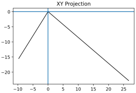
Note. The xy projection of the geometric space onto the relational contact space. 

This first orthogonal planar projection already demonstrates that at least one projection exhibits a contact graph difference. However, to be as rigorous as possible, we continue the application with the remaining 2 projections. 

Projection to 𝑥𝑧

𝑂𝑥𝑧(𝐶) = (−9.712,−0.906), and 𝑂𝑥𝑧(𝑆𝑐) = (26.677, 2.012) 

⟹ (176,190) = ‖𝑂𝑥𝑧(𝐶) ‖ =  = 9.754167314

⟹  (176, 190) = ‖𝑂𝑥𝑧(𝑆𝑐)‖ =  = 26.752765707

⟹ δ𝑥𝑧 = = 18.25346651 Å

⟹ (176, 190) ≤ δ𝑥𝑧< (176, 190) 

⟹ (176,190) ∈ 𝐸(, δ) and (176, 190) ∉ 𝐸(, δ) 

⟹ 𝐸(, δ) ≠ 𝐸(, δ) 

∴ 𝐺(, δ𝑥𝑧) ≠ 𝐺(, δ𝑥𝑧). 

Figure 3

xz Projection

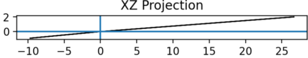
Note. The xz projection of the geometric space onto the relational contact space. 

Thus, there exists now a second planar projection where a graph invariance is observed (Figure  3). 

Projection to 𝑦𝑧 

𝑂𝑦𝑧 (𝐶) = (−15.540,−0.906), and 𝑂𝑦𝑧 (𝑆𝑐) = (−22.801,2.012) 

⟹ (176, 190) = ‖𝑂𝑦𝑧 (𝐶) ‖ =  = 15.566388 

⟹ (176, 190) = ‖𝑂𝑦𝑧 (𝑆𝑐)‖ =  = 22.8895991 

⟹ δ𝑦𝑧 = = 19.22799355 Å 

⟹ (176, 190) ≤ δ𝑦𝑧  < (176, 190)   

⟹ (176,190) ∈ 𝐸(,δ) and (176, 190) ∉ 𝐸(, δ) 

⟹ 𝐸(,δ) ≠ 𝐸(, δ) 

∴ 𝐺(, δ𝑦𝑧 ) ≠ 𝐺(, δ𝑦𝑧 ). 

Figure 4

yz Projection

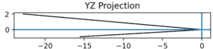
Note. The yz projection of the geometric space onto the relational contact space. 

The three orthogonal planar projections (Figures 2–4) show that regardless of which chosen planar coordinates of the witness pair (176, 190) that you will find a discrepancy between their embeddings. This further enforces the original claim of the structural conformation having vastly different structures. 

Interpretation 

We leverage several key implementations of metric space calculations in the ℝ¹, ℝ² and  ℝ³ proofs. Beginning with the initial proof in ℝ1, the concept was introduced of projecting a protein structure into its sequence-based representation. This framework relied on the assumption that both the infectious fibril and the non-infectious version of the major prion protein isoforms are simply expressions of PrP, and that neither protein was assumed to possess terminal edges within their globular domains. Due to the limitations of experimental structural biology methods and their inability to fully resolve atomic positions in flexible protein structures such as PrP, the applied proof in ℝ¹ required stripping the terminal residues of PrPᶜ and PrPˢᶜ and using only  purely the backbone of the residues representing the globular domain in the native PrPᶜ. This truncated sequence space representing the intersection of experimentally resolved residues was then shown to be equivariant using invariances. In other words, there was no way to tell the difference between MPP, 𝐶, 𝑆𝑐 given solely their backbone sequence code. Because we cannot differentiate the isoforms in ℝ¹, we use the experimentally observable difference in structure as an assumption to show through proof in ℝ³ that the structures are indeed different. 

The proof in ℝ³ was designed to show that each contact graph of the proteins had at least one delta which denoted a fixed midpoint for the edge sets to be derived from and allowed for a distance variance to be determined. This was further established in the applied proof where we use the 3D coordinates space from the mmCIF files to calculate the atom distances in PrPᶜ and PrPˢᶜ (Table 1). 

Table 1

Coordinates for Witnessed Non-Local Residue Pairs in PrPC and PrPSc

Structure	Residue	X (Å)	Y(Å)	Z(Å)
1QLX	176	-10.486	-14.457	-1.843
1QLX	190	-0.774	1.083	-0.937
6LNI	176	205.776	211.731	243.361
6LNI	190	179.099	234.532	241.349

Note. The 1QLX  and 6LNI structures provide the coordinates for PrPᶜ and PrPˢᶜ, respectively. The X, Y, and Z  coordinates expressed in Ångstroms (Å) for the residues 176 and 190 composing the witnessed  non-local residue pair in the application of proofs. 

The coordinates of the witnessed non-local pair in both PrPᶜand PrPˢᶜ structures give the ability to determine through a Euclidean norm that there is a midpoint for the set of intersecting residues representing the native globular domain. We can then use this midpoint as the anchor for distance projection. The distance projection reveals key differences between the two proteins; specifically, when we examine the midpoint delta, only one protein isoform satisfies the projected inequality, such that witnessed pair (176,190) remains within the edge set for the PrPᶜ isoform. 

To further demonstrate that there is a difference between the two isoforms, we use the ℝ2 proof to accomplish a projection that successfully reduces the dimensions of witnessed non-local  residue pair and thus simplifies computations. We perform a reduction in dimensional space such that, when analyzing any two planar projections of a three-dimensional structure, we can establish that there will be at least one view within that spatial reduction that demonstrates the witnessed pair does not exist in either edge set, and therefore in neither graph projection. This incongruity in graph projections is confirmed for every 3D planar projection in ℝ3regardless of dimensional combination. This further strengthens the claim that there exists a conformational difference between PrPᶜ and PrPˢᶜ. 

Discussion 

As this paper currently stands, there is very little addition to biochemistry,  stereochemistry, biophysics, combinatorics, or ionic interaction theory. This will be addressed in the ‘Further Research’ portion of this paper. Currently, this is an analysis of the basest level that observes sequence variation and applied that onto a 3-dimensional structural space, and that  allows for an ability to show a difference in physical properties. The addition of ionic interaction theories as well as proton channels that help regulate cell pH in the CNS is actively being  considered as well as further structural analysis of the fibril that PrPˢᶜ creates and signaling  effects in the host neuron.

Conclusion 

A key conclusion from this study is that the edge sets in the contact graphs do represent interacting partners, defined by the chosen distance thresholds between the witnessed residue pairs. However, the presence of an edge does not automatically imply a functional or causative interaction; for example, residues that are distant in the structure may or may not influence protein behavior through allosteric mechanisms, while more local contacts are likely to be more directly relevant. The observed differences in contact graphs reflect how these interactions act as structural variables and are incrementally modified, rather than providing a direct mapping to ionic interaction theory, biophysical interactions, or conformational dynamics. Importantly, this model aligns with current physical observations that the two forms of the major prion protein,  PrPᶜ and PrPˢᶜ, are structurally distinct, despite having identical primary sequences. 

Further Research 

This paper presents findings from ongoing research conducted by Ashley L. Bennett, PhD, and Nicole L. Mazuroski, M.S. Moving forward, this study proposes to incorporate electrostatic and ionic interaction principles to better understand protein conformational dynamics.  Specifically, it is hypothesized that metabolic stressors may induce a localized decrease in pH within the central nervous system, leading to an increased concentration of free hydrogen ions promoting protonation of key amino acid residues and inducing backbone conformational changes through altered salt bridge interactions. Additionally, interacting partners of PrPᶜ, may further modulate the local proton environment. For example, zinc may influence neuronal acidity by interfering with proton transport mechanisms, potentially reducing proton efflux, and contributing to intracellular proton accumulation. There is also ongoing discussion about the potential intracellular interactions of calcium, chloride, and copper, although these ideas remain speculative at this stage. 

---

References 

Anand, Uttam; Patra, Shubhadeep; Sekar, Rohith Vedhthaanth; Garen, Craig R.; & Woodside, Michael T. (2025). Different folding mechanisms in prion proteins from mammals with different disease susceptibility observed at the single-molecule level. Proceedings of the National Academy of Sciences, 122(29). https://doi.org/10.1073/pnas.2416191122

Andre, Ralph & Tabrizi, Sarah J. (2012). Misfolded PrP and a novel mechanism of proteasome inhibition. Prion, 6(1), 32–36. https://doi.org/10.4161/pri.6.1.18272

Artikis, Efrosini; Kraus, Allison; Caughey, Byron. (2022). Structural biology of ex vivo mammalian prions. Journal of Biological Chemistry, 298(8), 102181.https://doi.org/10.1016/j.jbc.2022.102181

Blumenthal, Leonard M. (1953). Theory and applications of distance geometry (1st ed.). Oxford at the Clarendon Press. https://archive.org/details/theoryapplicatio0000leon/page/n7/mode/2up

Boon Seng Wong; Liu, Tong; Li, Ruliang; Pan, Tao; Petersen, Robert B.; Smith, Mark A.; Gambetti, Pierluigi; Perry, George; Manson, Jean C.; Brown, David R.; Sy, Man Sun . (2001). Increased levels of oxidative stress markers detected in the brains of mice devoid of prion protein. Journal of Neurochemistry, 76(2), 565–572. https://doi.org/10.1046/j.1471-4159.2001.00028.x

Brown, David R. (2001). Copper and prion disease. Brain Research Bulletin, 55(2), 165–173. https://doi.org/10.1016/s0361-9230(01)00453-1

Brown, David R.; Qin, Kefeng; Herms, Jochen; Madlung, Axel; Manson, Jean; Strome, Robert; Fraser, Paul E.; Kruck, Theo; von Bohlen, Alex; Schulz-Schaeffer, Walter; Giese, Armin; Westaway, David; & Kretzschmar, Hans (1997). The cellular prion protein binds copper in vivo. Nature, 390(6661), 684–687. https://doi.org/10.1038/37783

Canoyra, Sara; Marín-Moreno, Alba; Espinosa, Juan Carlos; Fernández-Borges, Natalia; Vidal, Enric; Orge, Leonor; Benestad, Sylvie L.; Andréoletti, Olivier; & Torres, Juan María (2025). Classical BSE emergence from Nor98/atypical scrapie: Unraveling the shift vs. selection dichotomy in the prion field. Proceedings of the National Academy of Sciences, 122(29). https://doi.org/10.1073/pnas.2501104122

De La Rosa, Victor; Bennett, Ashley L.; & Ramsey, I. Scott. (2018). Coupling between an electrostatic network and the Zn2+ binding site modulates Hv1 activation. The Journal of General Physiology, 150(6), 863–881. https://doi.org/10.1085/jgp.201711822

Diestel, Reinhard. (2025). Graph theory. Springer.

Edgeworth, Julie Ann; Jackson, Graham S.; Clarke, Anthony R.; Weissmann, Charles; & Collinge, John. (2009). Highly sensitive, quantitative cell-based assay for prions adsorbed to solid surfaces. Proceedings of the National Academy of Sciences, 106(9), 3479–3483. https://doi.org/10.1073/pnas.0813342106

Gogte, Kalpshree; Mamashli, Fatemeh; Herrera, Maria Georgina; Kriegler, Simon; Bader, Verian; Kamps, Janine; Grover, Prerna; Winter, Roland; Winklhofer, Konstanze F.; & Tatzelt, Jörg. (2024). Topological confinement by a membrane anchor suppresses phase separation into protein aggregates: Implications for prion diseases. Proceedings of the National Academy of Sciences, 122(1). https://doi.org/10.1073/pnas.2415250121

Hirsch, Morris W. (1997). Differential topology (Corr. 6. print). Springer.

James, Thomas L.; Liu, He; Ulyanov, Nikolai B.; Farr-Jones, Shauna; Zhang, Hong; Donne, David G.; Kaneko, Kiyotoshi; Groth, Darlene; Mehlhorn, Ingrid; Prusiner, Stanley B.; & Cohen, Fred E. (1997). Solution structure of a 142-residue recombinant prion protein corresponding to the infectious fragment of the scrapie isoform. Proceedings of the National Academy of Sciences, 94(19), 10086–10091. https://doi.org/10.1073/pnas.94.19.10086

Matoušek, Jirí. (2002). Lectures on discrete geometry. Springer.

Kamali-Jamil, Razieh; Vázquez-Fernández, Ester; Tancowny, Brian; Rathod, Vineet; Amidian, Sara; Wang, Xiongyao; Tang, Xinli; Fang, Andrew; Senatore, Assunta; Hornemann, Simone; Dudas, Sandor; Aguzzi, Adriano; Young, Howard S.; & Wille, Holger. (2021). The ultrastructure of infectious L-type bovine spongiform encephalopathy prions constrains molecular models. PLOS Pathogens, 17(6), e1009628. https://doi.org/10.1371/journal.ppat.1009628

Kawauchi, Akio. (2011). Topology of prion proteins: A joint work with Kayo Yoshida. In Special Session on Knotting in Linear and Ring Polymer Models [Conference]. AMS Sectional Meeting. https://user.keio.ac.jp/~ishikawa/tms2011/files/tms2011_kawauchi.pdf

Kovač, Valerija; & Čurin Šerbec, Vladka (2022). Prion Protein: The Molecule of Many Forms and Faces. International Journal of Molecular Sciences, 23(3), 1232. https://doi.org/10.3390/ijms23031232

Kraus, Allison; Hoyt, Forrest; Schwartz, Cindi L.; Hansen, Bryan; Artikis, Efrosini; Hughson, Andrew; Raymond, Gregory J.; Race, Brent; Baron, Gerald S.; & Caughey, Byron. (2021). High-resolution structure and strain comparison of infectious mammalian prions. Molecular Cell, 81(21). https://doi.org/10.1016/j.molcel.2021.08.011

Lee, John M. (2013). Introduction to smooth manifolds (2. edition). Springer.

Masone, Antonio; Zucchelli, Chiara; Caruso, Enrico; Lavigna, Giada; Eraña, Hasier; Giachin, Gabriele; Tapella, Laura; Comerio, Liliana; Restelli, Elena; Raimondi, Ilaria; Elezgarai, Saioa R.; De Leo, Federica; Quilici, Giacomo; Taiarol, Lorenzo; Oldrati, Marvin; Lorenzo, Nuria L.; García-Martínez, Sandra; Cagnotto, Alfredo; Lucchetti, Jacopo; Gobbi, Marco; Vanni, Ilaria; Nonno, Romolo; Di Bari, Michele A.; Tully, Mark D.; Cecatiello, Valentina; Ciossani, Giuseppe; Pasqualato, Sebastiano; Van Anken, Eelco; Salmona, Mario; Castilla, Joaquín; Requena  Requena; Banfi, Stefano; Musco, Giovanna; Chiesa, Roberto. (2023). A tetracationic porphyrin with dual anti-prion activity. iScience, 26(9), 107480. https://doi.org/10.1016/j.isci.2023.107480

De Berg, Mark; Cheong, Otfried; & Overmars, Mark. (2008). Computational geometry: Algorithms and applications (3rd ed). Springer.

Miranzadeh Mahabadi, H., Hajar & Taghibiglou, Changiz.(2020). Cellular Prion Protein (PrPc): Putative Interacting Partners and Consequences of the Interaction. International Journal of Molecular Sciences, 21(19), 7058. https://doi.org/10.3390/ijms21197058

Ruffin, Vernon A.; Salameh, Ahlam I.; Boron, Walter F.; & Parker, Mark D. (2014). Intracellular pH regulation by acid-base transporters in mammalian neurons. Frontiers in Physiology, 5. https://doi.org/10.3389/fphys.2014.00043

Wang, Li-Qiang; Zhao, Kun; Yuan, Han-Ye;, Wang, Qiang; Guan, Zeyuan; Tao, Jing; Li, Xiang-Ning; Sun, Yunpeng; Yi, Chuan-Wei; Chen, Jie; Li, Dan; Zhang, Delin; Yin, Ping; Liu, Cong; & Liang, Yi (2020). Cryo-EM structure of an amyloid fibril formed by full-length human prion protein. Nature Structural & Molecular Biology, 27(6), 598–602. https://doi.org/10.1038/s41594-020-0441-5

Watt, Nicole T.; & Hooper, Nigel M. (2003). The prion protein and neuronal zinc homeostasis. Trends in Biochemical Sciences, 28(8), 406–410. https://doi.org/10.1016/s0968-0004(03)00166-x

Westergard, Laura; Christensen, Heather M.; & Harris, David A. (2007). The cellular prion protein (PrPC): Its physiological function and role in disease. Biochimica et Biophysica Acta (BBA) – Molecular Basis of Disease, 1772(6), 629–644. https://doi.org/10.1016/j.bbadis.2007.02.011

Wille, Holger & Requena, Jesús. (2018). The Structure of PrPSc Prions. Pathogens, 7(1), 20. https://doi.org/10.3390/pathogens7010020

Zahn, Ralph; Liu, A., Lührs, T., Riek, R., Von Schroetter, C., López García, F., Billeter, M., Calzolai, L., Wider, G., & Wüthrich, K. (2000). NMR solution structure of the human prion protein. Proceedings of the National Academy of Sciences, 97(1), 145–150. https://doi.org/10.1073/pnas.97.1.145

Zhang, Yongbo; Swietnicki, Wieslaw; Zagorski, Michael G.; Surewicz, Witold K.; & Sönnichsen, Frank D. (2000). Solution Structure of the E200K Variant of Human Prion Protein. Journal of Biological Chemistry, 275(43), 33650–33654. https://doi.org/10.1074/jbc.C000483200